Signal Processing

THREE_DECADES_VCO

Published:2009/7/1 21:01:00 Author:May

  (View)

View full Circuit Diagram | Comments | Reading(682)

SIMPLE_VOLTAGE_CONTROLLED_OSCILLATOR

Published:2009/7/1 21:00:00 Author:May

With the component values shown, the oscillator has a frequency of 8 kHz. When an input signal is applied to the base of Q1 the current flowing through Q1 is varied, thus varying the time required to charge C1. Due to the phase inversion in Q1 the direction of output frequency change is 180 degrees out of phase with the input signal. The output may be used to trigger a bistable flip-flop.   (View)

View full Circuit Diagram | Comments | Reading(914)

VOLTAGE_CONTROLLED_OSCILLATOR

Published:2009/7/1 20:59:00 Author:May

The VCO circuit, which has a nonlinear transfer characteristic, will operate satisfac-torily up to 200 kHz. The VCO input range is effective from1/3 VCC to VCC - 2 V, with the highest control voltage producing the lowest output frequency.   (View)

View full Circuit Diagram | Comments | Reading(229)

PRECISION_VOLTAGE_CONTROLLED_OSCILLATOR

Published:2009/7/1 20:58:00 Author:May

RC 4151 precision voltage-to-frequency converter generates a pulse train output linearly proportional to the input voltage.   (View)

View full Circuit Diagram | Comments | Reading(2186)

Liquid_flowmeter_thermally_based

Published:2009/7/24 3:25:00 Author:Jessie

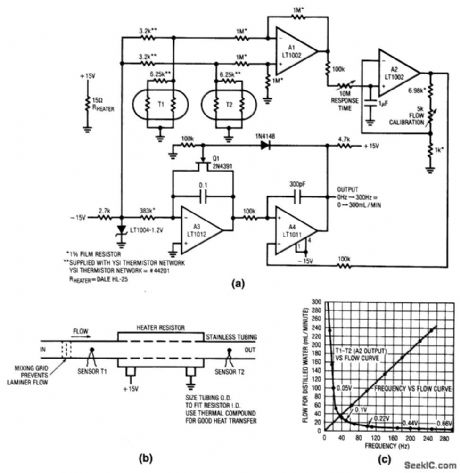
Fig. 14-3 This circuit shows a thermally based flowmeter, which features highly accurate rates as low as 1 mL/min and has a frequency output, which is a linear function of flow rate. This design measures the differential temperature between two sensors (Fig. 14-3B). Sensor T1, located before the heater resistor, assumes the fluid's temperature before the fluid is heated by the resistor. Sensor T2 picks up the temperature rise that is induced into the fluid by the resistor. The sensor difference signal appears at the Al output. A2 amplifies this difference with a time constant set by the response time adjustment. Figure 14-3C shows A2 output versus flow rate. The curves shown are for distilled water. To calibrate, set a flow rate of 10 mL/min and adjust the flow calibration trim for 10-Hz output. Linear Technology Linear Applications Handbook 1990 p AN5-6.   (View)

View full Circuit Diagram | Comments | Reading(696)

Accelerometer_digitizer_piezoelectric

Published:2009/7/24 3:21:00 Author:Jessie

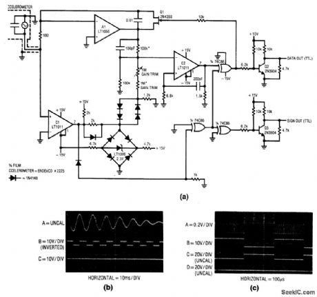
Fig. 14-1 This circuit is essentially a current-to-frequency converter that responds to ac input developed by an accelerometer, As shown In Fig. 14-1B, the piezoelectric accelerometer produces a damped sine-wave when subjected to acceleration (Trace A). This signal is converted to a signal output (Trace B), which keeps track of acceleration polarity. The frequency output (Trace C)supplies amplitude data. Note the drop In output frequency as the accelerometer wave-form damps. To trim, apply a known amplitude acceleration to the transducer and adjust the gain trim for the correct output frequency, Notice that the transducer manufacturer'datasheet shows means of simulating acceleration electrically, and it includes the necessary scale factors, Linear Technologv Linear Applications Handbook 1990 p AN-15,-16.   (View)

View full Circuit Diagram | Comments | Reading(1692)

10_Hz_TO_10_kHz_VOLTAGE_CONTROLLED_OSCILLATOR

Published:2009/7/1 20:47:00 Author:May

  (View)

View full Circuit Diagram | Comments | Reading(709)

LINEAR_VOLTAGE_CONTROLLED_OSCILLATOR

Published:2009/7/1 20:46:00 Author:May

The linearity of input sweepvoltage versusoutput frequency is significantlyimproved by using an op amp.   (View)

View full Circuit Diagram | Comments | Reading(0)

TANGENTIAL_WAVEFORM_GENERATOR

Published:2009/7/24 3:38:00 Author:Jessie

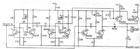
Generates approximation of tangent function for slant-range correction of video signal fromairborne infrared scanner. Ramp mvbr Q5-Q6 and timing mvbr Q1-Q2 are triggered simultaneously.-J. L. Woika, Generating Tangential Sweeps for Infrared Mapping, Electronics, 34:41, p 64-66.   (View)

View full Circuit Diagram | Comments | Reading(533)

10_MHz_fiberoptic_receiver_signal_conditioner

Published:2009/7/24 3:38:00 Author:Jessie

Fig. 14-10 This circuit accurately conditions a wide range of light-signal inputs at data rates up to 10 MHz. The circuit has both analog and digital outputs, as well as an analog output to monitor the detector. The digital output features an adaptive threshold trigger, which accommodates varying signal intensities (because of component aging, etc.). A test circuit is also included on Fig. 14-10. No calibration is required, Linear Technology Linear Applications Handbook 1990, p AN13-23.   (View)

View full Circuit Diagram | Comments | Reading(463)

Photodiode_signal_conditonerfrepuency_output

Published:2009/7/24 3:36:00 Author:Jessie

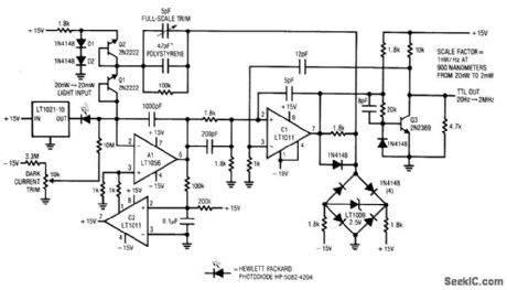
Fig. 14-9 This circuit converts a photodiode current output into an output frequency with 100 dB of dynamic range. Optical input power of 20 nW to 2 mW produces a linear 20-Hz to 2-MHz output. To calibrate the conditioner, place the photodiode in a completely dark environment and adjust the dark current trim so that the circuit oscillates at the lowest possible frequency, typically 1 or 2 Hz. Next, apply(or electrically simulate using the manufacturer's datasheet for light-input Versus output-current data)a 2-mW optical input. Adjust the full-scale trim capacitor for a 2-MHz output. If the adjustment is outside the range of the trimmer, alter the 47-pF value appropriately, Once calibrated, this circuit will maintain 1% accuracy(limited by the photodiode characteristics), Linear Technology Linea Applications Handbook 1990, p. AN7-9.   (View)

View full Circuit Diagram | Comments | Reading(690)

Humidity_to_frequency_converter

Published:2009/7/24 3:30:00 Author:Jessie

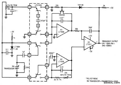
Fig. 14-6 This circuit converts the output of a relative-humidity (RH) transducer into a calibrated frequency output, using an LTC1043 switched-capacitor IC. To calibrate, place the transducer in a 5% RH environment, and adjust the 5% RH trim for 50-Hz output. Next, place the transducer in a 90% RH environment, and adjust the 90% RH trim for a 900-Hz output. Repeat this procedure unti1 both points are fixed. Relative humidity accuracy will be 2% over the 5%-90% RH range. If RH standards are not available, the circuit can be approximately calibrated with fixed capacitors in place of the transducer. Ideal values are 5% RH=379.3 pF and 90% = 523.8 pF. Note that these values assume an ideal sensor. An actual device can depart from the values by as much as 10%. Linear Technology Linea Applications Handbook 1990 p AN7-11.   (View)

View full Circuit Diagram | Comments | Reading(515)

Linearized_methane_transducer_signal_conditioner

Published:2009/7/24 3:28:00 Author:Jessie

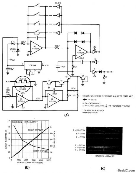
Fig. 14-5 The frequency output of this circuit is directly proportional to the methane concentration detected by the transducer. Figure 14-5B shows the transducer versus circuit response. To calibrate, place the transducer (sensor) in a 1000-pprn methane environment, and adjust the 1000-ppm trim for a 100-Hz output. Accuracy from 500 to 10,000 ppm is limited by the sensor 10% specification. Linear Technology, Linear Applications Handbook 1990. p AN11-3.   (View)

View full Circuit Diagram | Comments | Reading(513)

Thermal_anemometerair_flowmeter

Published:2009/7/24 3:27:00 Author:Jessie

Fig. 14-4 This circuit provides a voltage output that corresponds to airflow. The circuit operates by measuring the energy required to maintain a heated resistance wire at constant temperature. The sensor is a type 328 lamp with the glass envelope removed. The lamp is placed in a bridge monitored by A1. The A1 output is amplified by Q1 and fed back to the bridge. When power is applied, the lamp is at low resistance and the Q1 emitter tries to go full-on. As current flows through the lamp, the filament temperature rises quickly, which increases filament resistance. This increases the A1 negative input. A1 acts to balance the bridge by applying more current through Q1. Thus, the voltage at the Q1 emitter is predictably related to airflow past the lamp. The remaining circuits square and amplify the Q1 emitter voltage to give a linear, calibrated output versus airflow rate, To calibrate, place the lamp in the air flow so that the filament is at a 90° angle to the flow. Next, either shut off the air flow or shield the lamp from the flow, and adjust the zero flow for a circuit output of 0 V. Then, expose the lamp to air flow of 1000 ft/min and adjust the full-scale flow for 10-V output. Repeat these adjustments until both points are fixed. With this calibration, the air flowmeter is accurate within 3% over the entire 0- to 1000-ft/min range. Linear Technology Linear Applications Handbook, 1990, p. AN5-7.   (View)

View full Circuit Diagram | Comments | Reading(2552)

Photodiode_signal_conditioner_voltage_output

Published:2009/7/24 3:34:00 Author:Jessie

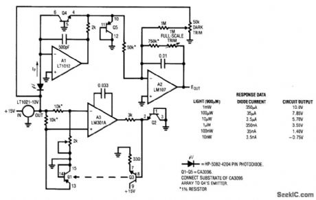
Fig. 14-8 This circuit converts the output of a PIN photodiode to a corresponding voltage. The specified photodiode responds linearly to light intensity over a 100-dB range. To accommodate this wide range without digitizing (this would require an A/D with 17 bits of range) the circuit compresses the photodiode output logarithmically (using the logarithmic relationship between VBE and collector current of transistors). This VBE/current relationship is temperature sensitive, and generally requires special layout of components. The circuit overcomes the layout problem because all transistors in the circuit are part of a CA3096 array. To calibrate, first set the thermal control loop by grounding the Q3 base and setting the 2-kΩ pot so that the A3 inverting input is 55 mV above the noninverting input. This places the servo setpoint at about 50℃ (assuming a 25℃ ambient). Remove the Q3 base ground and place the photodiode in a completely dark environment. Adjust the dark trim so that the A2 output is 0 V. Then, apply (or electrically simulate, using the chart) 1 mW of light (350μA of diode current) and set the full-scale trim for a 10-V output. Once adjusted, this circuit responds logarithmically to light inputs from 10 to 1 mW with an accuracy that is limited by the 1% photodiode error. Linear Technology Linear Applications Handbook 1990 p AN5-3.   (View)

View full Circuit Diagram | Comments | Reading(1370)

Level_transducer_digitizer

Published:2009/7/24 3:32:00 Author:Jessie

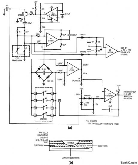
Fig.14-7 This circuit converts the angle(from an ideal level)to a corresponding frequency using a simple bubble-based transducer such as shown in Fig 14-7B．The circuit also provides a sign output(+ or -)to show either side of ideal level.If the transducer (bubble tube) is level with respect to gravity, the bubble is at the tube center and the electrode resistances to common are identical. As the tube shifts away from level, the resistances increase and decrease proportionally. By controlling the tube shape at manufacture, it is possible to get a linear output signal when the transducer is incorporated into a bridge circuit. To calibrate, place the level transducer at a known 40 arc-minute angle and adjust the calibrate potentiometer (at C1B) for a 400-Hz output. Circuit accuracy is limited by the transducer to about L5% Linear Technology Linear Applications Handbook l990, p. ANl7-12, -23.   (View)

View full Circuit Diagram | Comments | Reading(582)

Sampled_strain_gauge_conditioner

Published:2009/7/24 3:42:00 Author:Jessie

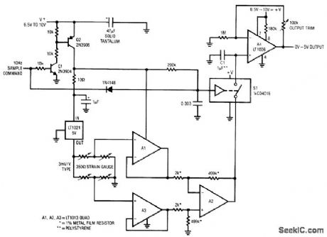
Fig, 14-13 This circuit converts the output of a strain-gauge to a corresponding voltage, but with considerable power savings produced by sampling. An external 10-Hz sampling signal or command is required. Effective current drain is about 300μA, and the A4 output is accurate enough for 12-bit systems. The 100-kΩ output trim pot is suitable for 3 mV/V transducers, but it might require a different value for other transducers, Linear Technology Linear Applications Handbook, 1990 AN23-3.   (View)

View full Circuit Diagram | Comments | Reading(649)

Pressure_transducer_conditioner

Published:2009/7/24 3:41:00 Author:Jessie

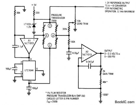
Pig. 14-12 This circuit converts the output of a pressure transducer to a voltage and it provides a 1.2-V reference output to a monitoring A/D converter for ratiometric operation (0.1 mA max/min). The circuit converts the bridge differential output into a ground-referred single-ended signal, which is then amplified. This approach eliminates common-mode errors by eliminating the bridge common-mode output component. No precision resistor matching is required. To calibrate, apply (or electrically simulate) 0 psi, and adjust the zero trim for 0-V output. Then, apply (or electrically simulate) 350 psi and adjust the gain trim for 3.500-V output. Repeat these adjustments until both points are fixed. Linear Technology Linear Applications Handbook 1990 p AN11-7.   (View)

View full Circuit Diagram | Comments | Reading(533)

Strain_gauge_conditioner_digitizer

Published:2009/7/24 3:40:00 Author:Jessie

Fig. 14-11 This circuit converts the dc output of a classic strain-gauge transducer to a frequency (actually a ratio of two frequencies). For a typical 7.5-μV strain-gauge bridge drive, an LSB increment is 25 μV (below most conventional A/D converters). The circuit data output (the ratio of output A to the clock frequency) can be extracted with counters. Because the output is expressed as a ratio, clock-frequency stability is unimportant. However, careful layout and a clean PC board are required. Use a teflon standoff for all summing-point connections. If a particular strain-gauge transducer requires zero trimming, use the optional network. Over a 0 to 70℃ range, the circuit typically maintains a 10-bit output with 1 LSB accuracy. The tracking error of the starred resistors are the primary contributors to this small error. No calibration is required. Linear Technology Linear Applications Handbook, 1990. p AN7-6.   (View)

View full Circuit Diagram | Comments | Reading(1629)

TIMING_PULSE_GENERATOR

Published:2009/7/1 20:06:00 Author:May

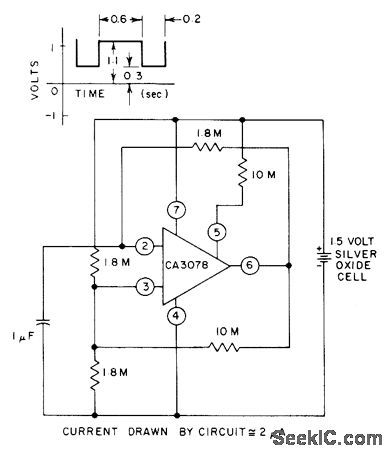
Astable MVBR uses CA3078 micropower opamp to develop timing pulses for driving other low-power circuits. Current drain is only about 2μA from 1.5-VDC supply.- Circuit ideas for RCA Linear ICs, RCA Solid State Division, Somerville, NJ, 1977, p 4.   (View)

View full Circuit Diagram | Comments | Reading(587)

Pages:123/195 At 20121122123124125126127128129130131132133134135136137138139140Under 20